My Awesome CSCI 0451 Blog

Perceptron

In this blog post I implement a perceptron. A perceptron is a funky little learning algorithm that only converges when data is linearly separable. It works by iterating over the points and only adjusting its weights when it is iterating over a point that is incorrectly labeled.

Walking through `Perceptron.fit`:

I am going to go over in order all of the lines of code that I believe to be the most noteworthy.

First X and y are modified to make them easier to work with.

X_ = np.append(X, np.ones((n, 1)), 1)
y_ = (2 * y) - 1

Then w is initialized to random values.

self.w = np.random.randint(-6, 6, X_.shape[1])

With those set we can start looping over points. To select points, every iteration a completely random point is selected from the dataset. As a result, it is very highly likely that some points will be iterated over multiple times before others have been looked it.
From there, it is possible to update the weights in one line, but I have broken it up for ease of understanding. The first step is making the prediction for the single data point by dotting w and that data point’s features.
```
y_pred = np.sign(np.dot(self.w, X_[i]))
```
Then, we check if that prediction is correct with some nice math.
```
false_check = (y_[i] * y_pred) < 0
```
Lastly, we use false_check as a gate to only update w if the prediction was incorrect. If the prediction was incorrect, this step moves the weights in the direction we want to go.
```
self.w = self.w + false_check * (y_[i] * X_[i])
```

from perceptron import Perceptron

import numpy as np
import pandas as pd
import seaborn as sns
from matplotlib import pyplot as plt

from sklearn.datasets import make_blobs

def draw_line(w, x_min, x_max):
  x = np.linspace(x_min, x_max, 101)
  y = -(w[0]*x + w[2])/w[1]
  plt.plot(x, y, color = "black")

Experiment 1: Linearly Separable 2D Data

This experiment looks at linearly seperable data with 2 features. The perceptron is able to quickly find a line that achieves 100% accuracy.

np.random.seed(12345)
n = 100
p_features = 3

X, y = make_blobs(n_samples = 100, n_features = p_features - 1, centers = [(-1.8, -1.9), (1.6, 1.7)])

p = Perceptron()
p.fit(X, y, steps=1000)

fig = plt.scatter(X[:,0], X[:,1], c = y)
fig = draw_line(p.w, -2, 2)

xlab = plt.xlabel("Feature 1")
ylab = plt.ylabel("Feature 2")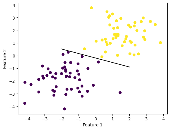

fig = plt.plot(p.history)
xlab = plt.xlabel("Iteration")
ylab = plt.ylabel("Accuracy")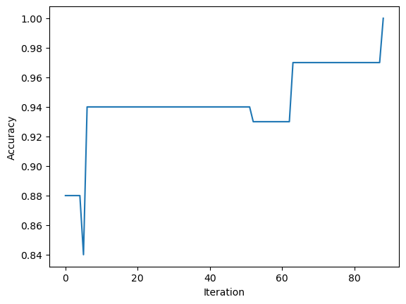

Experiment 2: NOT Linearly Separable 2D Data

This experiment looks at data with 2 features that is not linearly seperable. The perceptron is not able to find a set of weights (a line) that can accuractely predict all of the data points because the data because this data is not linearly seperable.

Also, one of the qualities of the perceptron is that it does not converge, and we can see in the graph below containing the accuracies over the iterations that the accuracy continues to jump up and down until it reaches the max number of steps.

np.random.seed(54321)
n = 100
p_features = 3

X, y = make_blobs(n_samples = 100, n_features = p_features - 1, centers = [(-1, -1), (1, 1)])

p = Perceptron()
p.fit(X, y, steps=1000)

fig = plt.scatter(X[:,0], X[:,1], c = y)
fig = draw_line(p.w, -2, 2)

xlab = plt.xlabel("Feature 1")
ylab = plt.ylabel("Feature 2")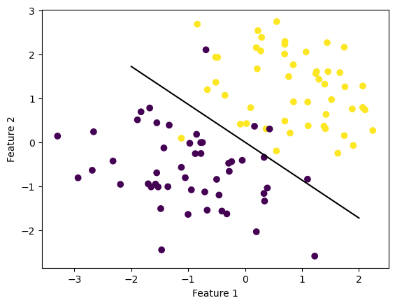

fig = plt.plot(p.history)
xlab = plt.xlabel("Iteration")
ylab = plt.ylabel("Accuracy")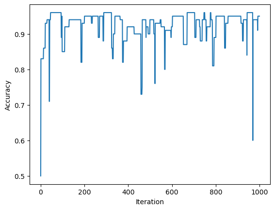

Experiment 3: Linearly Separable (?) 5D Data

This data containing 5 features turns out to be linearly seperable. We can tell it is linearly seperable without visualizing it because the perceptron is able to find line weights that make predictions with an accuracy of 100%.

np.random.seed(12321)
n = 100
p_features = 6
X, y = make_blobs(n_samples = 100, n_features = p_features - 1, centers = [(-1.75, -1.75), (1.75, 1.75)])

p = Perceptron()
p.fit(X, y, steps=1000)

fig = plt.plot(p.history)
xlab = plt.xlabel("Iteration")
ylab = plt.ylabel("Accuracy")

This data is linearly seperable. The perceptron was able to achieve 100% accuracy!

Runtime Complexity of the Update Step

The update contains multiple individual steps occuring in sequence. We will look at them all individually

First lets look at making the prediction: np.sign(np.dot(self.w, X_[i])). This operation does a 1xp dot px1 operation. This specific step is O(p).

Next, lets look at the forming of the gate: (y_[i] * y_pred) < 0. This is clearly O(1).

Now for the update: self.w + false_check * (y_[i] * X_[i]). The major component here is the scalar * vector operation. Since the vector is of length p, this is O(p) as well.

We could end there and be done, but we check the overall accuracy as part of the update step: (np.dot(self.w, X_.T) > 0). This is a dot product operation of 1xp vector and a pxn matrix. Therefore, this step has a runtime of O(pn).