from kernel_logreg import KernelLogisticRegression

import numpy as np
from matplotlib import pyplot as plt
from mlxtend.plotting import plot_decision_regions
from scipy.optimize import minimize
from sklearn.datasets import make_blobs, make_circles, make_moons
from sklearn.metrics.pairwise import rbf_kernelKernel Logistic Regression
In this blog post I have implemented kernel logistic regression. Kernel logistic regression is a lot like regular linear logistic regression except we modify the data beforehand in order to still be able to use linear regression on nonlinear data.
For those that are curious, my loss function remains largely unchanged. I simply use the kernel matrix instead of the regular nxp data matrix. I use all numpy functions that performs the operations on all of the rows.
np.seterr(all='ignore')

def draw_line(w, x_min, x_max, color="black", ax=None, alpha=1):
    x = np.linspace(x_min, x_max, 101)
    y = -(w[0]*x + w[2])/w[1]
    if ax is None:
        plt.plot(x, y, color = color, alpha=alpha)
    else:
        ax.plot(x, y, color = color, alpha=alpha)

def construct_plot(X, y, clf, ax=None, title="Accuracy = "):
    plot_decision_regions(X, y, clf=clf, ax=ax)
    if ax is None: ax = plt.gca()
    title = ax.set(title = f"{title}{(KLR.predict(X) == y).mean()}",
                        xlabel = "Feature 1",
                        ylabel = "Feature 2")
Experiments
Experiment 1: Basic Check
Here I am just confirming that all of my code actually works.
Running a test on moon shaped data with gamma=0.1 I get a model that is a pretty good fit for both train and test data.
X_train, y_train = make_moons(200, shuffle = True, noise = 0.2)
KLR = KernelLogisticRegression(rbf_kernel, gamma = .1)
KLR.fit(X_train, y_train)

X_test, y_test = make_moons(100, shuffle = True, noise = 0.2)
fig, (ax1, ax2) = plt.subplots(1, 2, figsize=(12, 6))

construct_plot(X_train, y_train, KLR, ax1, "Training Accuracy = ")
construct_plot(X_test, y_test, KLR, ax2, "Test Accuracy = ")
Experiment 2: Choosing Gamma
In this experiment I will demonstrate the importance of choosing a good gamma value. A gamma too low will underfit the data, but a gamma too high will overfit the data. As we can see values for gamma above 1 begin to lose accuracy on the test set.
X_train, y_train = make_moons(80, shuffle = True, noise = 0.2)
X_test, y_test = make_moons(80, shuffle = True, noise = 0.2)
gammas = [.01, .1, 1, 10, 100, 1000, 10000]
fig, axarr = plt.subplots(len(gammas), 2, figsize=(12, 6*len(gammas)))

for i, gamma in enumerate(gammas):
    KLR = KernelLogisticRegression(rbf_kernel, gamma=gamma)
    KLR.fit(X_train, y_train)
    construct_plot(X_train, y_train, KLR, axarr[i][0], f"gamma={gamma} Training Accuracy = ")
    construct_plot(X_test, y_test, KLR, axarr[i][1], f"gamma={gamma} Test Accuracy = ")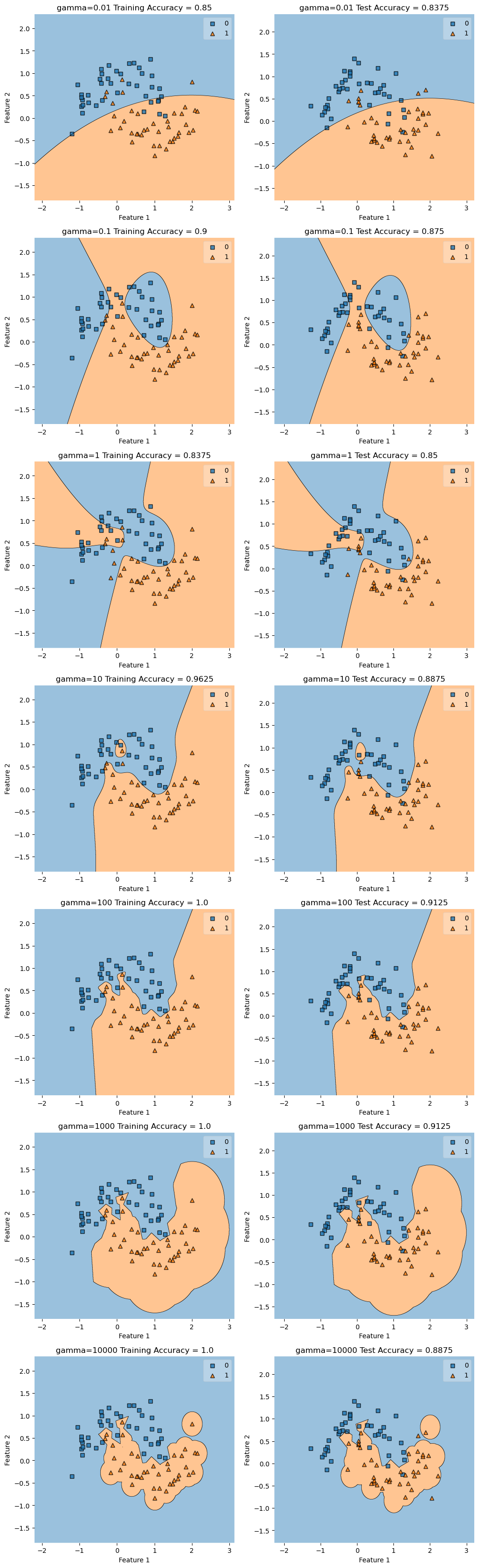
Experiment 3: Varied Noise
In this experiment I vary the noise paramater of the make_moons function, and I test what values of gamma are best with increased noise.
In the last experiment we tested with noise=.2 and saw that a gamma value of around 1 was sufficient.
Testing with Noise=.05
From this test we can gather that when there is very little noise (and very little difference between the train and test data), we just need a high enough gamma to follow the shape.
X_train, y_train = make_moons(80, shuffle = True, noise = 0.05)
X_test, y_test = make_moons(80, shuffle = True, noise = 0.05)
gammas = [.01, .1, 1, 10]
fig, axarr = plt.subplots(len(gammas), 2, figsize=(12, 6*len(gammas)))

for i, gamma in enumerate(gammas):
    KLR = KernelLogisticRegression(rbf_kernel, gamma=gamma)
    KLR.fit(X_train, y_train)
    construct_plot(X_train, y_train, KLR, axarr[i][0], f"gamma={gamma} Training Accuracy = ")
    construct_plot(X_test, y_test, KLR, axarr[i][1], f"gamma={gamma} Test Accuracy = ")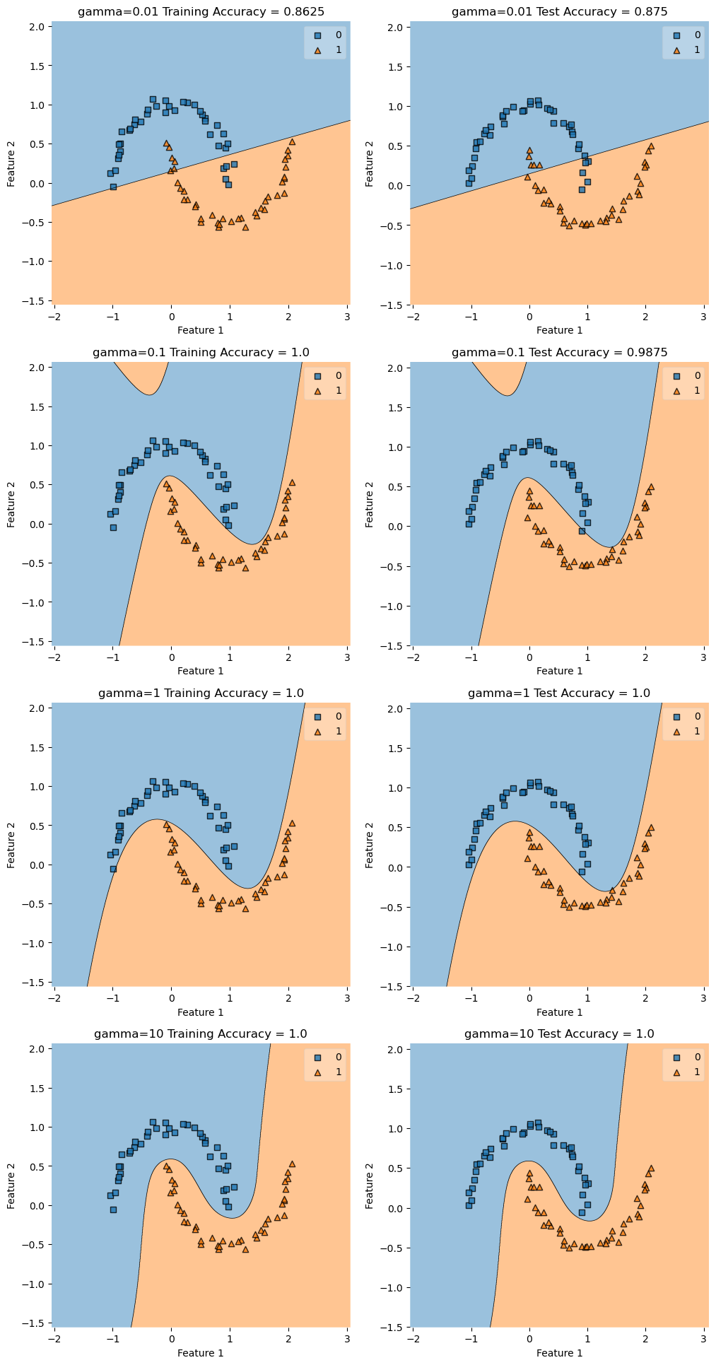
Testing with Noise=.04
In this test we see that a gamma of .1 does a the best at matching the shape we want. Higher than .1 is overfit and below .1 is underfit.
X_train, y_train = make_moons(80, shuffle = True, noise = 0.4)
X_test, y_test = make_moons(80, shuffle = True, noise = 0.4)
gammas = [.01, .1, 1, 10]
fig, axarr = plt.subplots(len(gammas), 2, figsize=(12, 6*len(gammas)))

for i, gamma in enumerate(gammas):
    KLR = KernelLogisticRegression(rbf_kernel, gamma=gamma)
    KLR.fit(X_train, y_train)
    construct_plot(X_train, y_train, KLR, axarr[i][0], f"gamma={gamma} Training Accuracy = ")
    construct_plot(X_test, y_test, KLR, axarr[i][1], f"gamma={gamma} Test Accuracy = ")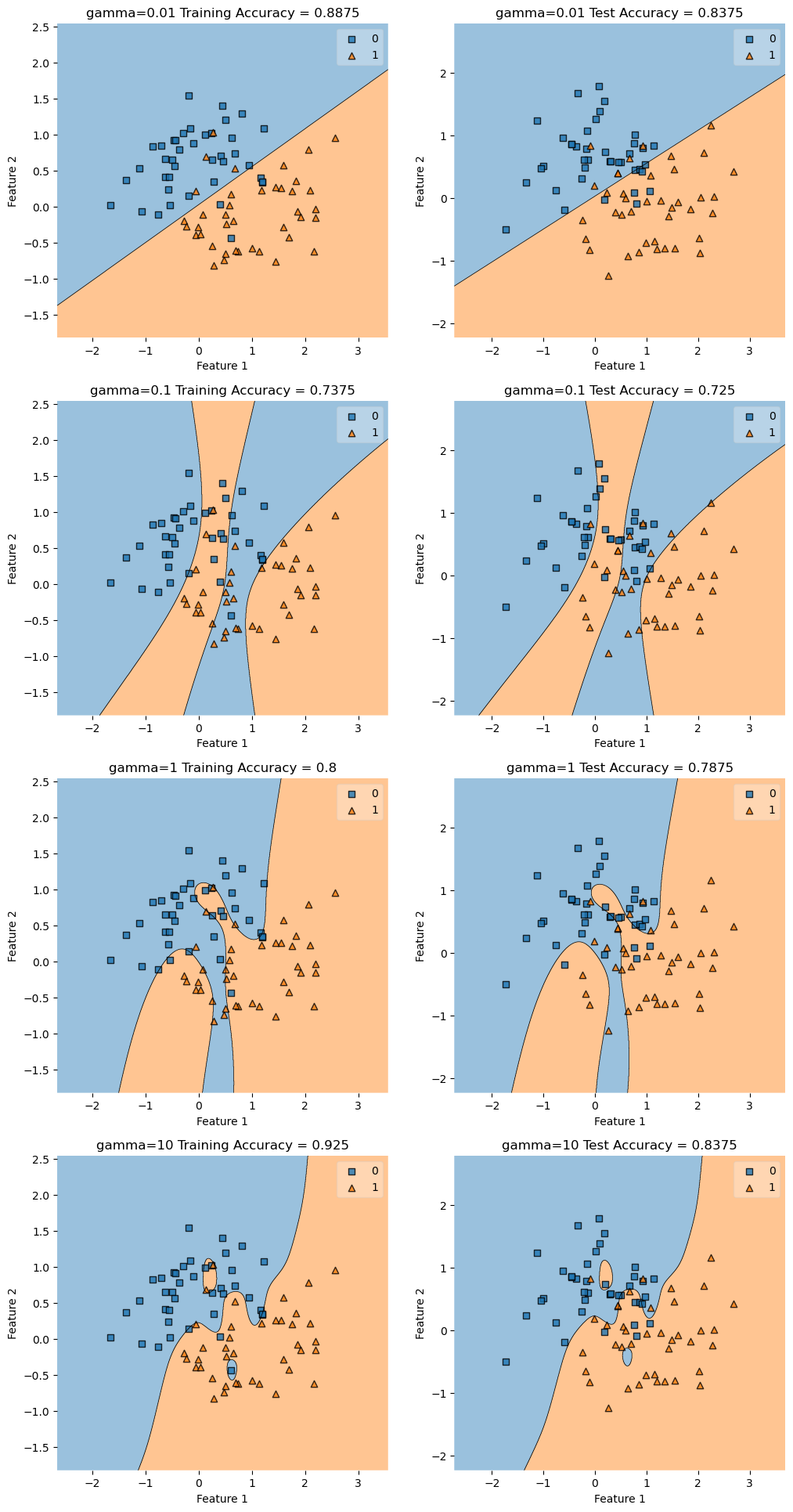
Conclusions from Experiment 3
Overall, I don’t have enough evidence to suggest that the best value for gamma depends on the noise level. This generally matches what I have seen in the documentation that assigns gamma based off of the size of the training set.
Experiment 4: Other Shapes
Testing with gamma=.1
noises = [0, .1, .2]
fig, axarr = plt.subplots(len(noises), 2, figsize=(12, 6*len(noises)))
gamma = .1
for i, noise in enumerate(noises):
    X_train, y_train = make_circles(50, shuffle = True, noise = noise)
    X_test, y_test = make_circles(50, shuffle = True, noise = noise)
    KLR = KernelLogisticRegression(rbf_kernel, gamma=gamma)
    KLR.fit(X_train, y_train)
    construct_plot(X_train, y_train, KLR, axarr[i][0], f"noise={noise} Training Accuracy = ")
    construct_plot(X_test, y_test, KLR, axarr[i][1], f"noise={noise} Test Accuracy = ")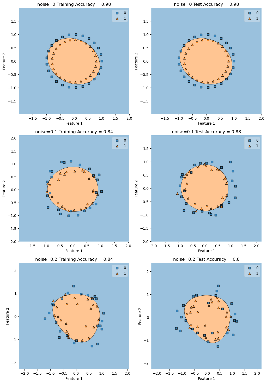
Testing with gamma=1
noises = [0, .1, .2]
fig, axarr = plt.subplots(len(noises), 2, figsize=(12, 6*len(noises)))
gamma = 1
for i, noise in enumerate(noises):
    X_train, y_train = make_circles(50, shuffle = True, noise = noise)
    X_test, y_test = make_circles(50, shuffle = True, noise = noise)
    KLR = KernelLogisticRegression(rbf_kernel, gamma=gamma)
    KLR.fit(X_train, y_train)
    construct_plot(X_train, y_train, KLR, axarr[i][0], f"noise={noise} Training Accuracy = ")
    construct_plot(X_test, y_test, KLR, axarr[i][1], f"noise={noise} Test Accuracy = ")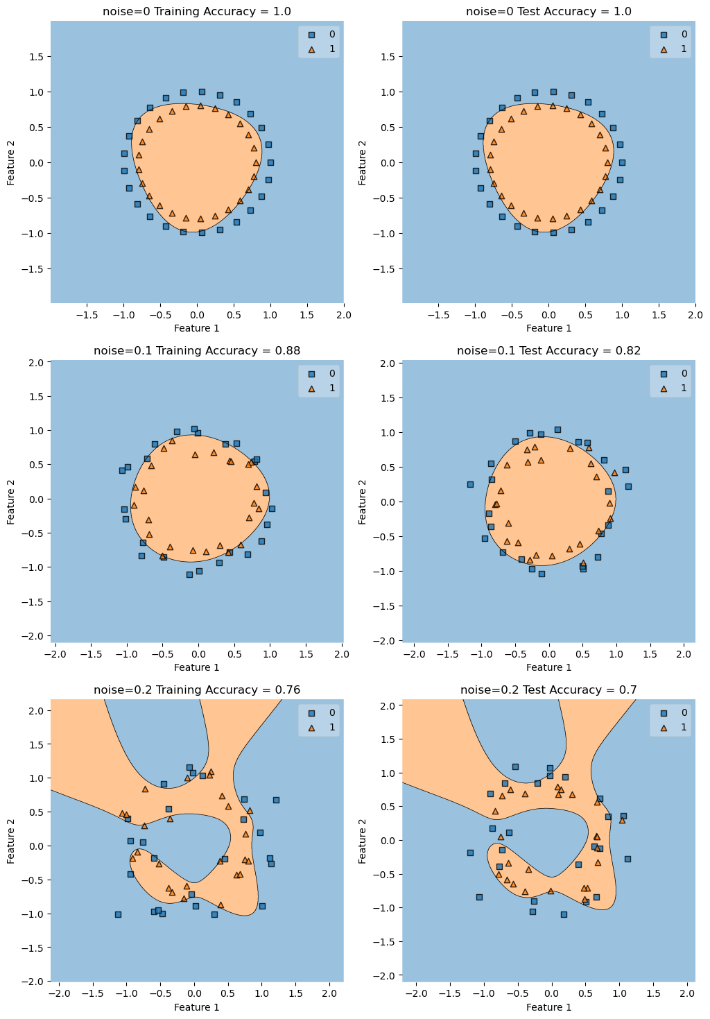
Testing with gamma=10
A gamma value of 10 is too high with
noises = [0, .1, .2]
fig, axarr = plt.subplots(len(noises), 2, figsize=(12, 6*len(noises)))
gamma = 10
for i, noise in enumerate(noises):
    X_train, y_train = make_circles(50, shuffle = True, noise = noise)
    X_test, y_test = make_circles(50, shuffle = True, noise = noise)
    KLR = KernelLogisticRegression(rbf_kernel, gamma=gamma)
    KLR.fit(X_train, y_train)
    construct_plot(X_train, y_train, KLR, axarr[i][0], f"noise={noise} Training Accuracy = ")
    construct_plot(X_test, y_test, KLR, axarr[i][1], f"noise={noise} Test Accuracy = ")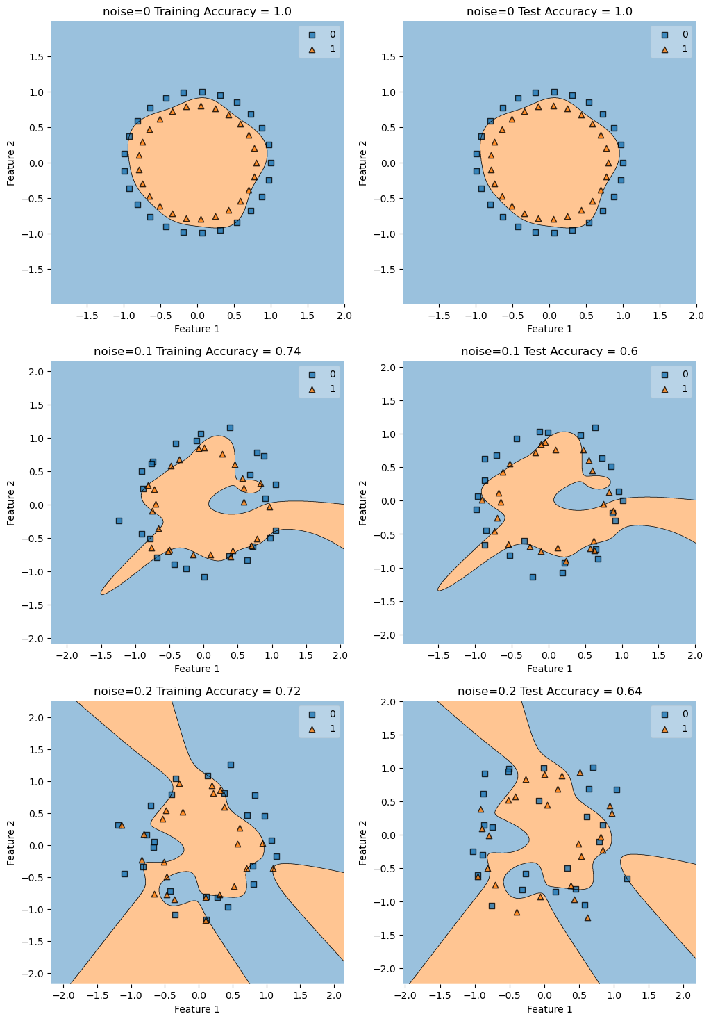
Conclusions from Experiment 4
When there is no noise pretty much any reasonable gamma will do, but once there starts to be signficant noise, the lower gamma value does better on this set.